The ultimate assignment, as in, the last one.

Our final assignment for my statistics for public managers class (#JSGS807) was to use an online data set to explore a policy issue of your choice and to create data visualizations.

My policy issue was to look at data surrounding opioid related deaths in Canada and to look at how Saskatchewan compares to other provinces and Canada as a whole.  Opioid related deaths have become a lot like cancer in that it seems like there are few families not affected by addiction to opioids and I’d hazard a guess that most people know someone that has passed on due to an overdose. Just in this past year, my best friend’s cousin whom I knew casually, lost her battle with addiction. Opioids ruled her life as well as her death.

Leaving the anecdotal behind, I looked to the Government of Canada’s report on “Apparent opioid-related deaths” and the Government of Saskatchewan’s data on
“Drug toxicity deaths between 2010 and 2018”.
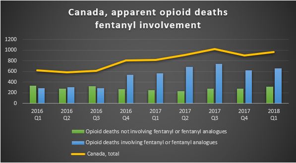
Table 1

Canada is facing an opioid crisis. In the last year and a half alone, opioid deaths have increased by 60 percent and the largest increase in this trend is due to fentanyl or fentanyl analogues being associated with the opioid used.

Looking at the opioid deaths by province; British Columbia, Ontario and Alberta had the highest number of deaths in 2016 and 2017…
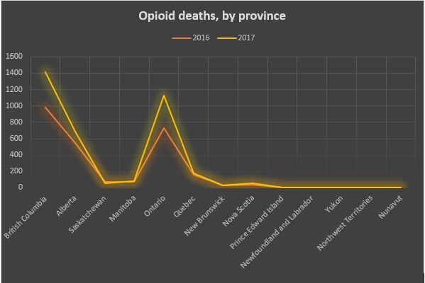
Table 2

… even though Quebec has the second highest population in Canada.
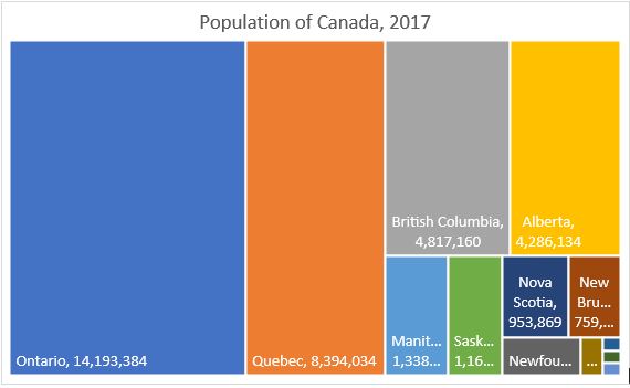
table 3

Why Quebec has a much lower number and rate of death due to opioids is interesting, but not part of my original question.  Are Quebec’s drug laws and policies such that even if addiction rates are similar, fewer people are dying?  If so, this may well point to strategies that could be considered to be adopted to reduce rates elsewhere,  but I still haven’t looked at my target, Saskatchewan.

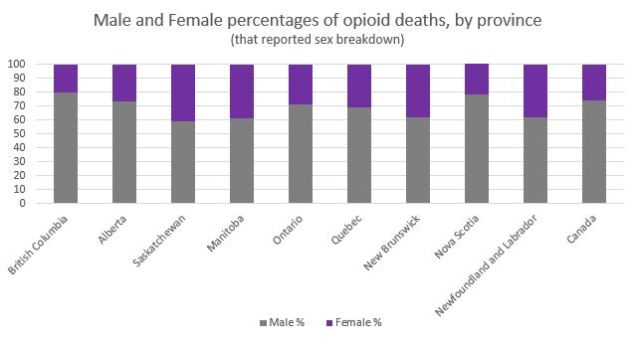
How does Saskatchewan compare to Canada overall and relative to its population size? Looking at population size, Saskatchewan is about on par with the other provinces with similar-sized populations.  But if you look at the breakdown of male and female opioid deaths for 2017, Saskatchewan is an outlier.
ta ble 4

Overall in Canada, females represent 26 per cent of opioid related deaths as seen by the purple sections above but in Saskatchewan in 2017, the percentage of female deaths related to opioids is 41 per cent, the highest in the country.  Saskatchewan has had the highest percentage of female opioid related deaths in Canada for the past 5 years.  Is it perhaps related to the manner of death?
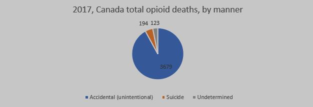
table 5

In 2017, the vast majority of opioid related deaths were ruled to be accidental overdoses. Looking at the National average, only 4.9 per cent of the deaths were ruled to be suicides. The data in that report held no further breakdown, so I looked to Saskatchewan’s data to see if I could see what was different about Saskatchewan.  While I did note that women were much more likely to commit suicide by intentional overdose in Saskatchewan, I did not have the data from other jurisdictions to compare this to so in the end I am left with questions and other paths to explore.

To continue looking at this, my next steps would be to see if I could find data sets that may help me understand why the female/male ratio for Saskatchewan is the highest in Canada and I would explore why Quebec’s death rates are so low.   If it isn’t an artificial difference in data (like differences in reporting) and is truly a much lower rate per 100,000 people in the province, there may be policies to adopt that would reduce the harm in Saskatchewan and in other jurisdictions.

Hey, not every wheel has to be invented from scratch, if you find a good policy, adopt it and apply it!

Looking at the process I used to examine the issue; well, it reminds me that I have a few basic beliefs that I use to guide my life.

Treat others as you’d like to be treated.

Don’t do anything you wouldn’t like to have broadcast (especially prudent now that life can be live streamed).

Assume you can do anything until experience teaches you that you should focus your energies elsewhere.

Producing analytics may well be one of those things that fall on the weaknesses side of the ledger for me. Knowing what your strengths and weaknesses are is half the battle and producing mind-blowing visualizations may not be one of my strengths. I spent more than 30 hours trying to download data sets, trying to format them into something I could use in Tableau, getting them into Tableau and then trying to produce something from them.  There is a lot of data out there, but little of it is ready to use as is.

What I learned from all of this (the assignment and the class) is that I will remember to have a deep appreciation for my data analytics team at work.  It isn’t easy!

I also learned from the class that even if I am not (currently) highly proficient at producing visualizations, I can be a better and more knowledgeable consumer of statistics, infographics and other visualizations.

But I haven’t given up on learning this skill. I am persistent if nothing else.
Are data visualizations just smoke and mirrors?

The overarching premise of a briefing note is to provide a recommended action or response to an issue based on the background and analysis of the issue, and the identification of the advantages and disadvantages of the options for action that are identified.   While notes may be brief, especially at the Minister’s level, there is still the requirement that good policy is evidence based and evidence generally involves data.

Not every briefing note requires the use of visualization techniques.  Even for more complex issues, evidence may be legislative or precedence based and while the issue may be complex, it may not require the use of statistics to point to an optimized action to be recommended.  Where visualizations become important is when the data you are working with is extensive or complex.

Especially in cases where there may be more than one tenable option, the issue is new, or the recommended option is innovative or counter to current practice, the analyst should use all of his or her skills to assist the governing body to make an appropriate decision.  These skills include knowing your audience, presenting your information in a clear and concise manner and recognizing when a visual representation of statistics or other data makes your information easier or quicker to understand.

In the case of a Minister’s note, using a visualization to reduce a wall of words or a huge table of data into a more concise format is assistive.   Whether or not you use visualizations or decide to stick to a more neutral presentation, what makes it assistive and not manipulative is the reason you make that choice.  You don’t need a visualization to obfuscate an issue; if your intent is to unduly influence someone, it can be done just as well with neutral but misleading or incomplete presentation of facts so while a visualization may be given a different weight than a bullet point or table of data, understanding when and why it is appropriate to relay information visually goes a long way towards ethical public policy.

Increasing your  POBU (probability of being understood)

There are challenges inherent in every type of communication and public policy is no different.   Public policy involves using evidence-based analysis to look at options, assess risks, and develop recommended actions based on the possible outcomes.

In the face of the current climate where the masses are bombarded with polarizing information in the guise of news or facts, evidence-based analysis is more important now than it has ever been.  It won’t sway the blinkered, but it will help public servants make defensible decisions on public policy.

Background information can involve measurement of the past and when measuring the past, you can be precise.  When you analyze and develop policy, you look at probabilities.

Take talking about the weather, for example.  It’s easy to understand the factual past in that Regina received 0.2 mm in the last 24 hours but in looking at the probability of precipitation (POP) for the next 24 hours, that level of precision would not be appropriate.  If people understood the calculation for the POP, they’d stop maligning the poor, misunderstood meteorologist.    The POP is the percentage of time that weather conditions just like the time period being forecast would result in precipitation, so a 60% POP means that if you had 10 days with exactly the same atmospheric conditions, you could expect precipitation to fall over some portion of the forecast area in 6 of 10 similar days.

The use of probabilities is also essential in the assessment of the risk associated with any policy.  Possible impact without an associated likelihood doesn’t show which risks to focus your mitigation strategies on.

But unless people (including you!) understand what you are trying to convey when you use probabilities, the use of probabilities is counterproductive.  Probability statements based on industry specific calculations such as POP are commonly misunderstood as people don’t understand the calculations that they are based on and people likely don’t look on the percentage in the same way that a meteorologist does.

Reduce the risk that your audience will be unable to properly assess likelihood by providing a definition that explains your probability statement within your analysis.  Policy doesn’t deal with the incontrovertible.  Increase your  POBU (probability of being understood)  through definition of terms that are commonly misunderstood.

All the best indicators make for a fine Index, the Best Index for indicating Wellness.

Perhaps the title of my blogpost is a bit of a spoiler alert to the outcome of the Health Employment Security Index (HESI) rankings but in case you can’t tell which country ranked number one on the HES index by the title I’ll spoil it fully now; it was the United States of America (USA).

In examination of the data indicators selected, it is fairly apparent why this isn’t really a ranking that tells anyone much but I’m sure there is at least one person south of the border that would consider this the unfakest news.  Is it on Fox News yet?

To construct the index, I selected four indicators across three dimensions.  My thoughts at the time were that the more secure a population is in having a minimum amount of education required to be employed, in being able to get a secure job, and living in a country that has significant spending on the healthcare system, the higher a country would score on the Health Employment Security Index.

Being employed in a job that isn’t exploitative and having healthcare available goes a long way to providing a sense of mental and physical health for me, perhaps it would do the same for others.

The indicators I chose were government health spending as a percentage of the country’s GDP, a composite indicator based on unemployment percentage and vulnerable employment percentage and finally, the percentage of the population over 25 that at has at least some secondary education.   I figured that blending unemployment with vulnerable employment would provide a measure of not only being employed but being employed in with an adjustment of how likely the job was a ‘good’ job.  Vulnerable employment includes self employed workers with no employees and people that work for family but are not at a level that would be considered a partner. They are less likely to have formal work arrangements, and are therefore more likely to lack decent working conditions.  As unemployment is a negative aspect and the other two dimensions had (what I considered to be) positive indicators, I used the inverse of the unemployment data to have all positive indicators contributing to the HESI.

The health spending indicator I had chosen had no data for 2017 and in fact, it was somewhat difficult to find indicators that comprehensively included most, if not all of the countries in the Human Development Index (HDI).  In order to not make this more complex than needed, I chose to stick with these indicators.  While three of the four indicators used data from 2017 for the most part, the health spending data was from 2015.  There were a few countries where I opted to use the most recent data in order to include them in the rankings.

Another issue was that for the dimensions using a single indicator, the country with the minimum score in the indicator had to be adjusted by 0.001 to allow for a geometric mean to be calculated for the index and I noted these by using red text in the data table.

The outcome was that the USA came out with the number one ranking.  This made me look at my assumptions and the data chosen as I think I’d feel very unwell in an employment/health way if I was in the USA.

Perhaps the health spending in the USA is so high because it is some of the most expensive healthcare in the world.  Perhaps countries have found a way to provide health care at a lower cost.

Looking at the two countries at the top of the HDI: Norway dropped from #1 on the HDI to #7 on the HESI, mainly due to mid-pack health spending relative to its GDP.  Switzerland predictably remained neutral.

Canada?  Canada rose from 12th place to 6th on the HESI due to a very high education score and a better than average employment score but was batting 500 on healthcare spending.

The country that gained the most in the rankings was Liberia where the ranking increased 107 spots!  The country that dropped the most in the rankings was Brunei Darussalam which dropped 117 spots between rankings and both of these were affected most by the country’s healthcare spending or lack thereof so it is likely this dimension would be better represented by another indicator or at least by blending this indicator with another one.

While the USA spends a lot of money on the most expensive healthcare system in the world and you are unlikely to have to work for your dad who won’t pay you anywhere near where you should be paid as long as you get some secondary schooling, this may not be the strongest wellness index on earth.  Sorry, DT.

Putting the fun back into function

Member engagement is a struggle for pension plans.  People put more time into researching their smartphone than they put into reviewing their pension and retirement plans in a year.   By the age that people start to pay attention to their retirement, there is not much time to make an adjustment, if needed, for a member to achieve the retirement they are expecting.

In an effort to engage younger pension plan members and interest them in looking at their retirement trajectory, we are proposing a simulated investment tool where plan members learn about the value of time, compounding interest through the gamification of a traditional retirement calculator can make a big difference to not only how but when they will be able to retire.   Before engaging members in their personal retirement estimates, grab their attention with a game that demonstrates the general concepts of a fictional account.

The proposed simulator would provide the member with choices along the way. Members would make choices such as whether to make voluntary contributions to their pension plan, various investment choices along the way (including the concept of the default glide path), and how decisions to split their disposable income between things, experiences and registered retirement products throughout their life can make a difference to how closely they need to pay attention to the cost of living where he or she plans to live in retirement or what they’ll do with their time.

By using gamification to take the stuffiness out of a traditional retirement calculator where people enter data and get graphs and charts back an provide younger members with a game where a member can ‘win’, our agency may be more likely to engage and educate younger plan members.

Uber easy?

Right up front I’ll say I’m not the type of person who would be likely to try and get by in a gig economy.  I have to know I have a next cheque coming and exactly how much that cheque will be.   This whole simulation stresses out this practical, stability-craving, rule follower.  Fortunately, I also have a complete lack of social life so would have no impediments to driving seven days a week so I was able to win, at least 30% of the time.

While the game supposes that you are trying to make enough money to make a $1000 mortgage payment using the sharing economy and Uber, you find out at the end of the game that you have to reduce your earnings by any expenses.  This include your car lease, a phone data plan, and insurance for the vehicle which I would agree are costs if you didn’t already have these things. While I’d definitely use these as income tax write-offs, I would consider that a positive amount and a bonus as I’d have incurred the cost of a vehicle and insurance whether I was Ubering or not.

The simulation is a ‘choose your story’ type of simulation where you make choices to advance the story.  Some choices will add to your expenses and some will add to your bottom line.  Others don’t change things much.  In the first scenario, whether you call Chris or not, the only difference is that you complete it three minutes earlier if you just wait.  But all other parameters remain the same.

The choices do reflect things you’d want to know or consider as a driver, keeping receipts, whether to fix a windshield chip right away but if it is based on real life fares and costs, I can’t imagine it being an easy way to make a living as I pretty much had to work 10 hours a day on average, seven days a week to hit my target.    I’m not sure the Uber Game teaches much about issues around the regulation of the sharing economy by governments but it may help government understand what the Uber drivers have to face.   Instead of looking at how to put the brakes on innovations that reduce consumption in society by encouraging the use of less by many, governments could look at the use of pilot projects, uptake-based caps for licences or other temporary regulations where data would help decide whether an innovative share is a societal assistance or a hindrance.

So while I may be personally boring and staid to the nth degree, I’m always open to innovation when something new makes sense.

It’s not as easy as it looks. Seriously.

For the first assignment in my Statistics for Public Managers class, we needed to use an online data set to calculate and graph descriptive statistics.

There is a lot of data out there but it isn’t all easily accessible and much of it doesn’t lend itself to statistical analysis very well.  I downloaded and perused a few types of data before settling on a file of data from the Government of Alberta.

The data set I finally examined was Alberta’s Blue Book data from the first quarter of the
2018-2019 fiscal year. It shows who is doing business with government and payments that have been made for supplies or services purchased by departments from the General Revenue Fund.

As I didn’t have a question up front, in my examination of the data, I analysed it I three different ways: by single transaction, by total payments per supplier, and by government department.

Payments ranged from a minimum amount which was a refund to the government of $171,000 to a maximum single payment of $181,163,819 making the range $181,334,819.  With 5073 payments ranging so broadly, and a single payment representing 12.6% of the spending recorded in the blue book for the quarter, I was not expecting a symmetrical distribution of size of payments.

stats 1

Even when the 5073 payments were totaled per unique supplier, the data included 2590 suppliers.  With the mode at the extreme lowest point of total payments to a single supplier and the median total payment per supplier in the quarter at less than 1/10th of the average total payment per supplier, it indicated an expected positive skew in the data.  Calculating the skew confirmed a large positive skew at 27.8.

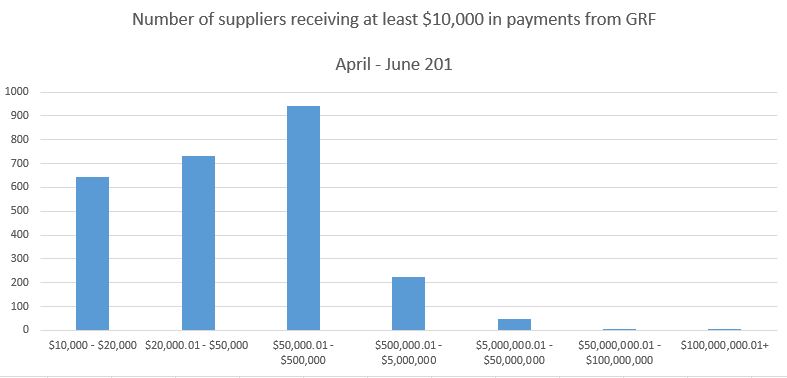
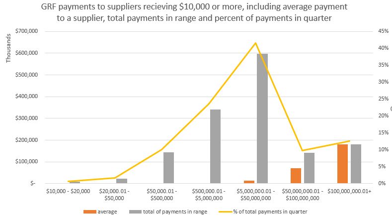
Grouping the payments by governmental department, 89.4% of all suppliers receiving at least $10,000 in the quarter received less than $500,000 and when combined, represented 36% of the total amount recorded for the quarter.  The other 10.6% of suppliers received 64% of the total in the quarter.

stats3

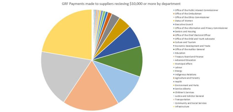
Comparing government departments to each other, the department spending the most was Infrastructure, and the three departments of Infrastructure, Community and Social Services, and Transportation made 58% of all payments.

stats2

In the end, I learned a lot about payments by departments in the Alberta Government in the first quarter of the 2018-2019 fiscal year and what you can and can’t do with descriptive statistics.

2 per cent smarter

Recently, I asked some of my friends, family and cohorts to help make me 2 per cent smarter and they responded in greater numbers than I expected.  I’m not sure what that says about their perception of me but I’m choosing to see it as a positive thing. My statistics assignment was to create and deploy a survey and I figured if I provided a fun hook to reel people in, I’d have a better chance at having people answer.  Here is what I did and what I learned.

While there was a bit of a learning curve on the software, it did provide options for different types of questions and options to make the survey more visually interesting than basic text-based surveys.

Writing the survey was interesting, as no matter how carefully you try to craft a question, it will never be crystal clear to everyone that reads it.  Using a different question type for every question is not likely a great idea.  At least not for 81-year-old moms.  But then again, she just learned to ‘text’ [Mom, it’s an iPad and it’s not texting when you use email or Facetime] so there is that.  But 81 year-old people may be a demographic you want to capture and if so, I would consider the ease of use for my target respondents if I was writing a survey.  It was actually hard to write questions that had no real purpose.  Having a clearly identified issue helps you form targeted questions.

I don’t have a large social media footprint but I tapped both Facebook and Twitter and I directly emailed a few of my friends to ask them to take the survey.  In a real research situation, I’d try for a much more random sample and a larger one but even with the small sample size, the statistical analysis that was provided by the software was interesting.  In the question where people had to rank foods from most liked to least liked, there were three foods that had large standard deviations that meant that people either loved or hated that food, it rarely fell in the middle.  The food with the lowest standard deviation from its mean was the lowly oyster, but only because it was almost universally disliked.

I was able to get what I consider to be a fair number of people to answer my survey by using a bit of humor to entice them in but it likely wouldn’t be a good technique in a real research situation as it could influence the participant’s mood or attitude towards the survey.

Statistics as the foundation of policy

I write briefing notes daily.  The influence involved in providing the information required and recommendations for actions to be taken by the trustees of a governing body to make significant and extensive decisions on the assets of public stakeholders is a responsibility I take very seriously.

A trustee holds assets on behalf of another and must do so in the beneficiary’s best interests.  The trustee makes decisions affecting those assets and must employ a duty of due diligence and a duty of care.

Public policy that is evidence based and rooted in good governance allows for decisions to be made with a standard of care that a prudent person would take and with the diligence brought through effective process. Statistical analysis is the foundation of evidence-based decisions, but statistics don’t provide evidence in and of themselves.   You need to understand how to interpret statistics to use them suitably.   Otherwise, recommendation of public policy based on statistics which are misunderstood or worse, intentionally misleading, is purely a justification for a position that likely isn’t in the best interest of all stakeholders affected by that decision.  When statistics are used appropriately, the allow the governing body to build a strong foundation in policy.